Advanced RF Analysis¶

Five analysis modules added in v4.1.5 that go beyond chamber-only metrics.

Link Budget / Range Estimation¶

Friis transmission with protocol presets (BLE, WiFi, LoRa, Zigbee, LTE, NB-IoT). Computes maximum range given TX power, antenna gains, frequency, and required SNR.

$$P_r = P_t + G_t + G_r - 20\log_{10}!\left(\frac{4\pi d}{\lambda}\right) - L_{\text{cable}}$$

Indoor Propagation¶

Implements ITU-R P.1238 (distance-power loss with floor-penetration factor) and ITU-R P.2040 (material penetration loss).

Environment presets: Office, Hospital, Industrial, Residential, etc. Each preset preloads the appropriate path-loss exponent.

Multipath Fading¶

Rayleigh and Rician CDF curves plus Monte-Carlo simulation. Useful for estimating margin in cluttered environments.

Enhanced MIMO¶

Capacity curves — Shannon capacity vs SNR with correlation effects
Combining gain — selection, equal-gain, maximal-ratio (verified math; see Math fixes)
MEG — Mean Effective Gain with XPR (cross-polarization power ratio)

Wearable / Medical¶

Body-worn pattern adjustments. Dense-device SINR. SAR screening estimator.

Math fixes (v4.0.0)¶

The original combining-gain formula was wrong. v4.0.0 verified:

Diversity gain uses the Vaughan-Andersen formula $DG = 10\sqrt{1-\text{ECC}^2}$ — NOT a log-based formula.
Combining gain validated against simulated MIMO-EVK data; agrees to within float precision (one pre-existing test still rounds 4.999… vs 5.0 — unrelated to physics).

Kraus efficiency caveat¶

Kraus formula:

$$\eta_{\text{Kraus}} = \frac{32400}{\text{HPBW}_E \cdot \text{HPBW}_H}$$

Only valid when both HPBW values ≤ 180°. RFlect rejects results that produce $\eta > 100\%$ — the assumption breaks for omnidirectional or low-directivity antennas.

Accessing these modules¶

Tools menu → Advanced RF Analysis. Sub-dialogs are scrollable since the parameter set is large.

There are currently no MCP wrappers for these modules. Open an issue if you need one — most are pure-Python in plot_antenna/advanced_* and could be wrapped quickly.

RF method gallery (v6.0)¶

The figures below are authentic outputs of the new v6.0 RF methods (plot_antenna/rf_methods.py, exposed as MCP tools). Regenerate them with python docs/generate_example_figures.py.

Uniform linear array — electronic beam steering¶

Array factor steering

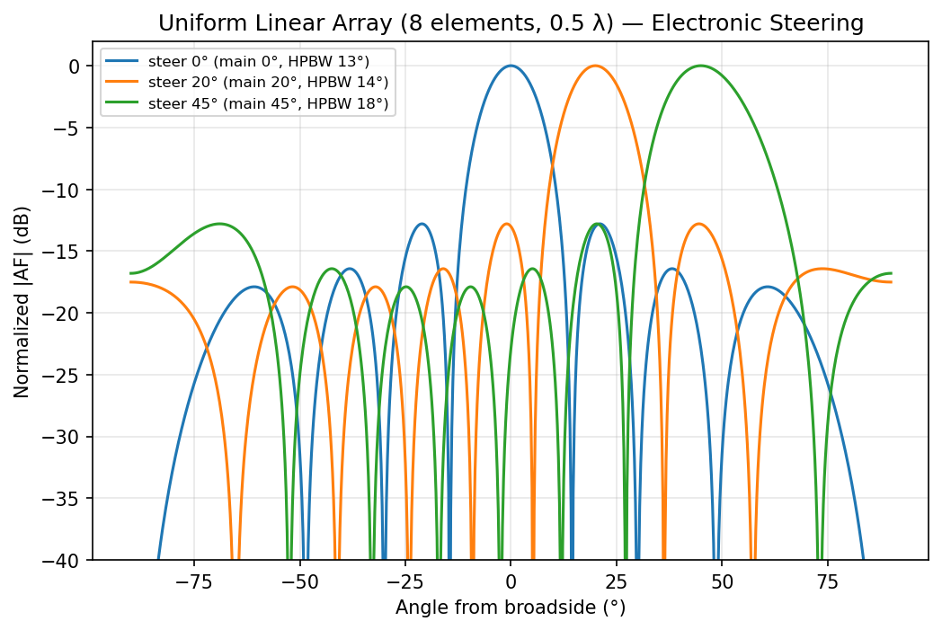
An 8-element, 0.5 λ array steered to 0°, 20°, and 45°. Note the main beam broadening (scan loss) as it steers off broadside — the reported HPBW grows from ~13° to ~18°.

Aperture taper trade-off¶

Array taper comparison

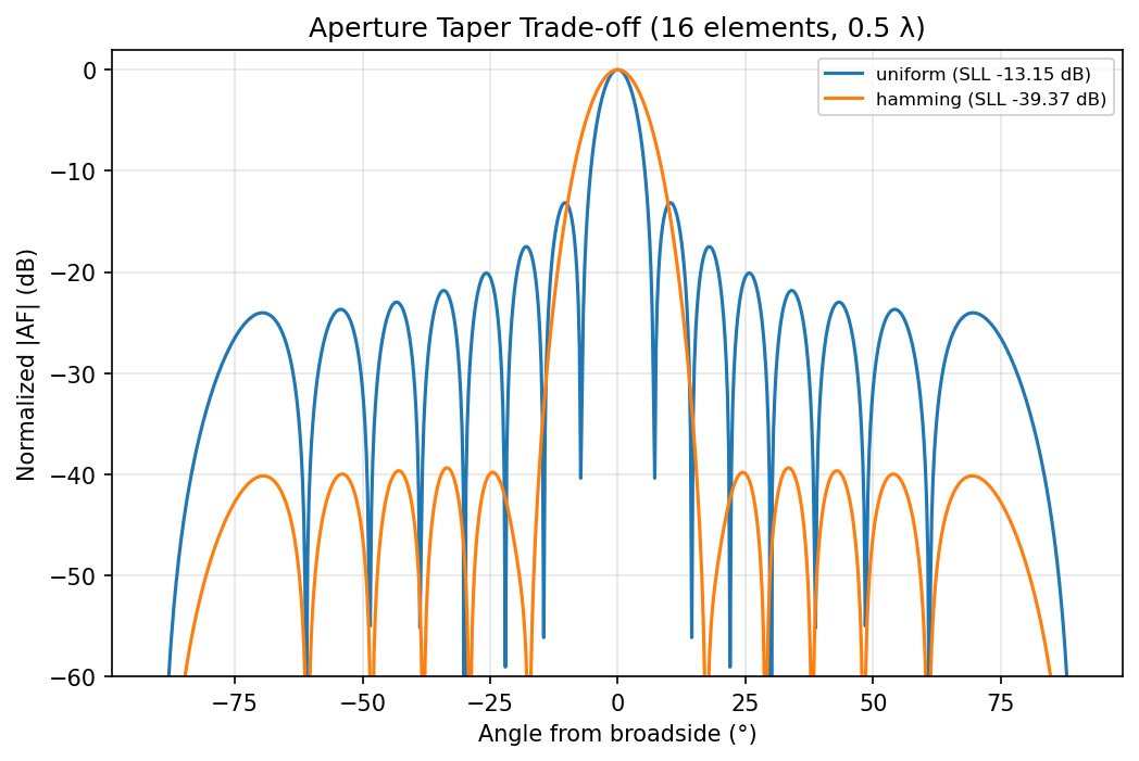
Uniform vs Hamming taper on a 16-element array: the taper trades ~3 dB of main-beam width for a large drop in peak sidelobe level.

Axial ratio vs H/V phase¶

Axial ratio sweep

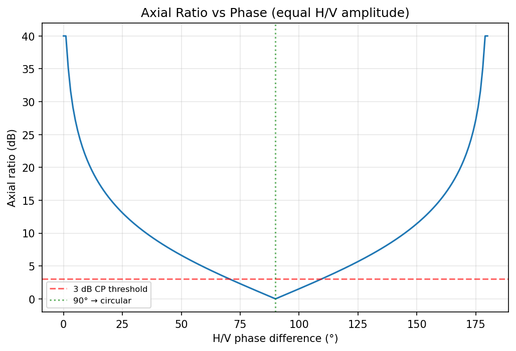
With equal H/V amplitude, axial ratio dips to 0 dB (perfect circular polarization) at a 90° phase difference and rises toward the linear-polarization asymptote at 0° and 180°. The 3 dB line marks the usual CP acceptance threshold.